Geoff Hulten - Machine Learning Course
Notes on a great course by Geoff Hulten on Machine Learning.
- Course web page
- Textbooks
- Tom M. Mitchell: Machine Learning
- Geoff Hulten: Building Intelligent Systems
- 1: Overview of Machine Learning
- slides
- D. Sculley et al: Machine Learning: The High-Interest Credit Card of Technical Debt (2014)
- Supervised learning \(Y=f(X)\):
- Discrete \(Y\): Classification
- Continuous \(Y\): Regression
- Probability Estimation: \(P(Y \vert X)\)
- Unsupervised, semi-supervised learning
- Reinforcement learning
- ML algorithm components
- Model structure
- Linear
- Decision trees
- Ensembles of models
- Instance based methods
- Neural nets
- Support vector machines
- Graphical models (Bayes/Markov nets)
- Etc
- Loss function
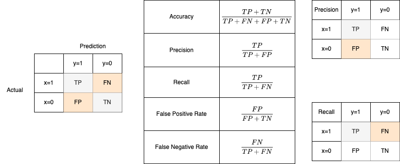
- Accuracy
- Precision & Recall
- Cost / Utility
- Squared error
- Likelihood
- Posterior probability
- Margin
- L1 & L2 normalization
- Entropy
- KL divergence
- Etc
- Optimization - how the learning algo finds the best model
- Greedy search
- Gradient descent
- Linear programming
- Regularization
- Look ahead, momentum, stochastic methods / batching, learning rates, termination conditions, etc
- Model structure
- Top 5 Career Paths for Data Professionals
- 2: Basics of Evaluating Models
- slides
- Training set, validation set, test set
- Overfit, underfit
- Confusion matrix
- 3: Logistic Regression
- slides
- Linear model for classification and probability estimation
- Can be effective when:
- The problem is linearly separable
- Or there are a lot of relevant features (10s-100s)
- Need efficient runtime or need a baseline
- Not the most accurate option, but used a lot in practice
- Model: linear with sigmoid activation \(\hat{y} = sigmoid(w_0 + \sum_{i=1}^n w_i * x_i)\) where \(sigmoid(x) = \frac{1}{1+e^x}\)
- Loss function: log loss \(Loss(\hat{y},y) = -y \, log(\hat{y}) - (1-y) \, log(1 - \hat{y})\)
- Optimization: gradient descent
- Parameters
- Step size used in gradient descent
- Convergence - minimum loss increase required to continue gradient descent
- Threshold - value between 0-1 to convert \(\hat{y}\) into a classification
- 4: Intro to Feature Engineering with Text
- slides
- Binary Features
- Contains word?
- Is SMS longer than X?
- Contains (*#)?
- Categorical Features
- First word is {noun, verb, other…}
- Message length is {short, medium, long, very long}
- Token type is {Number, URL, Word, Phone #, Unknown}
- Grammar Analysis is {Fragment, Simple Sentence, Complex Sentence}
- Numerical Features
- CountOf Word(call)
- MessageLength
- FirstNumberInMessage
- WritingGradeLevel
- Feature Engineering for words
- Tokenize
- Bag of words
- N-grams
- TF-IDF (term frequency - inverse document frequency)
- Embeddings - Word2Vec and FastText
- NLP
- Normalization of numeric features
- Feature engineering in other domains
- Computer vision
- Gradients
- Histograms
- Convolutions
- Internet
- IP Parts
- Domains
- Relationships
- Reputation
- Time series
- Window aggregation
- Frequency domain transformation
- Computer vision
- 5: Intro to Feature Selection
- slides
- Frequency
- Take N most common features in the training set
- Mutual information
- Take N features that contain most information about the value of Y on the training set
- Mutual information: \(MI(X,Y)=\sum_{x \in X, y \in Y}p(x,y) ln (\frac{p(x,y)}{p(x)p(y)})\)
- Accuracy
- Greedy search, add and remove features, evaluate on validation data
- 6: ROC Curves and Operating Points
- slides
- Logistic regression produces score between 0-1.
- Use threshold for classification
- Vary threshold to get best result
- Build Receiver Operating Characteristic (ROC) curve to plot False Negative Rate by False Positive Rate by threshold
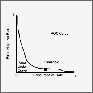
- AUC is area under curve, used for comparing performance between models. Operating point is point on ROC curve closest to origin. PR curve is same but for precision/recall. Update threshold to avoid drift. Threshold can be updated w/o having to update model.
- 7: Bounds and Comparing Models
- slides
- Tom M. Mitchell: Machine Learning Chap. 7
- Goal: predict how a model will behave once deployed
- Central limit theorem: if you have a population with mean \(\mu\) and standard deviation \(\sigma\) and take sufficiently large random samples from the population with replacement , then the distribution of the sample means will be approximately normally distributed with the same mean \(\mu\) and standard deviation \(\sigma\).
- \(x\%\) confidence interval defines a range of values that you can be \(x\%\) certain contains the population mean.
- IF: Better_Model – Bound > Worse_Model + Bound
- THEN: With \(x\%\) confidence the model that looks better on the sample is better
- ELSE: there is less than a \((1 - x \%)\) chance the model that looks worse is actually better
- Is new parameter or feature worth using?
- Train with or without feature
- Compare using one sided bounds
- Cross validation
- Split data into k folds
- Train with & without feature on k-1 folds
- Validate on remaining fold
- Use all validation data when computing bounds
- When to use cross validation? When you need to measure accuracy variance:
- For feature selection
- When data changes from under the model, causing variance
- When ML algorithm includes internal randomization, causing variance
- Be careful of data drift
- Time series
- Dependencies of data on other factors that may change (e.g. spam campaigns)
- Other violations of interdependence assumptions
- 8: Naive Bayes
- slides
- See Tom M. Mitchell: Machine Learning, Chap. 6.9
- Discriminative vs Generative modes
- Discriminative: model the posterior probability \(P(y \vert x)\) directly
- Use logistic regression, decision trees, neural nets
- Generative: model the joint probability \(P(x, y)\)
- Use naive Bayes, Bayesian networks, hidden Markov models
- On generative models: Andrew Y. Ng, Michael I. Jordan: On Discriminative vs Generative classifiers: A comparison of logistic regression and naive Bayes
- Discriminative: model the posterior probability \(P(y \vert x)\) directly
- Bayes Theorem: \(P(A \vert B) = \frac{P(B \vert A) P(A)}{P(B)}\)
- Bayes model: \(y = \underset{y_j \in Y}{argmax} \frac{P(\lt x \gt \vert y_j) P(y_j)}{P(\lt x \gt)}\)
- Same as \(y = \underset{y_j \in Y}{argmax} P(\lt x \gt \vert y_j) P(y_j)\)
- Simplifying assumption: the features \(x_i\) of \(\lt x \gt\) are independent (where the name ‘naive’ comes from)
- Naive Bayes model: \(y = \underset{y_j \in Y}{argmax} P(y_j) \underset{i}{\prod} P(x_i \vert y_j)\)
- Of theoretical importance, almost never used in practice
- For small number of features \(x_i\) and classes \(y_j\), build incidence table of how many times \(<x> \rightarrow y\), and compute \(y\) using naive Bayes
- 9: Implementing with Machine Learning
- 10: Decision Trees
- slides
- Tom M. Mitchell: Machine Learning Chap. 3
- 11: Defining Success with Machine Learning
- 12: Overfitting and Underfitting
- slides
- Inductive bias - assumptions you make about how likely any particular concept is
- Model structure
- Linear model
- Axis-aligned tree structure
- Labels are clustered
- Dataset selection
- Train/test/validate
- Cross validation
- Concept complexity
- Occam’s Razor - all other things being equal, simpler model is better
- Regularization
- Types of model errors
- Bias - caused when the model cannot represent the concept
- Variance - caused when the model overreacts to small changes in the data
- Noise - data was a bit corrupted; labels were a bit wrong, etc
- Total loss = bias + variance + noise
- Model structure
- 13: Intelligent User Experiences
- 14: Ensembles 1: Bagging & Random Forests
- slides
- Models can have bias or variance
- When models are too simple, they can’t represent complex concepts (bias)
- Complex models can overfit noise in data (variance/jitter)
- Ensembles: combine multiple models
- Can mitigate bias or variance
- Often result in better accuracy
- Approaches
- Use multiple independent models to learn, and combine the result randomly (bagging, random forest), or by using a meta-model to select result (stacking)
- Works for high variance, low bias base models
- Chain models, and use output error of previous model as input to next model, then combine the results (boosting, gradient boosting machines)
- Models in chain learn different parts of the concept
- Can work with high bias base models
- May overfit
- Use multiple independent models to learn, and combine the result randomly (bagging, random forest), or by using a meta-model to select result (stacking)
- Bagging
- Create $k$ training sets by sampling with replacement from original set
- Train $k$ independent models
- Combine predictions by uniform voting
- Each model learns concept a different way
- Bootstrap sampling accentuates variance between $k$ models
- Voting tends to cancel out variance without increasing bias
- Good when base models have low bias / high variance
- Boosted trees
- Same as bagging, but randomly drop features from each of the $k$ independent models
- Compared to bagging, feature restriction introduces higher variance
- 15: Ensembles 2: Boosting
- slides
- Create chain of models
- Model $i$ trained on residual error of model $i-1$
- Reweighting training data: give bigger weight to samples that had higher error
- Final result is weighted sum of intermediate results
- Stop adding models when starting to overfit (check on holdout set)
- Boosting can help with bias and variance, but can overfit.
- Gradient Boosting Machines (GBM) often used in practice to get high accuracy
- 16: Ensembles 3: Stacking & Intelligence Architectures
- slides
- Stacking: same as boosting, but train metalearner on holdout data to pick winner
- Organizing Intelligence is critical for long term success with ML
- Stacking (meta models)
- Business Logic
- Sequencing (sequence of models can eliminate junk according to own rules; simple to extend and maintain)
- Partitioning (break down into subproblems independently solved by different models)
- 17: ML Design Pattern: Adversarial Learning
- 18: Basics of Computer Vision
- 19: Neural Networks
- slides
- Tom M. Mitchell: Machine Learning Chap. 4
- 20: Neural Network Architectures
- 21: ML Design Pattern - Corpus Centric
- 22: Reinforcement Learning
- slides
- Tom M. Mitchell: Machine Learning Chap. 13
- 23: ML Design Pattern - Ranking