Yann LeCun - CDS Machine Learning Course
Notes on Deep Learning Course at CDS
05L - Joint embedding method and latent variable energy based models (LV-EBMs), slides
- Energy based models (EBM) vs Discriminative models
- Energy \(F(x, y)\), where \(x\) is observed variable, and we’d like to predict variable \(y\).
- Find \(\check(x)=argmin_y F(x, y)\) (energy is minimized)
- Choice of energy function does not matter if minimum is achieved for same value \(y\). For example, if we add a constant to \(F\), the minimum does not change.
- Can compute if \(y\) is discrete, or if there is a dynamic-programming-style way to compute \(y\)
- Energy \(F(x, y)\) computed during training
- If \(F\) is a smooth function of \(y\), can use gradient descent during inference to compute \(\check{y}\)

- Factor Graphs
- Conditional EBM: \(F(x, y)\) has conditional variable \(x\)
- Unconditional EBM: \(F(y)\). Here, \(x\) does not exist.
- PCA
- k-means clustering
- Any unsupervised algorithm can be cast as unconditional EBM
- Both \(x\), \(y\) are inputs to model \(F\).
- Connection to probabilistic models
- Probabilistic models are special case of EBM
- Energies are like un-normalized negative log probabilities
- Why use EBM instead of probabilistic models?
- EBM gives more flexibility in
- Choice of scoring function
- Choice of objective function for learning
- EBM gives more flexibility in
- From energy to probability: Gibbs-Boltzmann distribution
- Softmax is an instance of the Gibbs-Boltzmann distribution
- You pick \(\beta\), it is arbitrary
- For physicists, this constant is aking to temperature.
- The exponential makes numbers positive. Gives high values to low energy (which is what you want - likely configurations have low energy)
- Denominator is normalization factor
- LeCun does not say it - but \(P(y \vert x)\) can be seen as number of configurations with energy \(F(x, y)\) (but normalized)
- Compare with Statistical mechanics - a set of lectures, R. Feynman (1981), 1st lecture where he derives Boltzmann’s equation in statistical mechanics from properties of energy and temperature
- Energy function is like a cost we want to minimize
- Inference becomes optimization problem to find \(y\)
EBM architectures:
- Joint embeddings
- Variational models
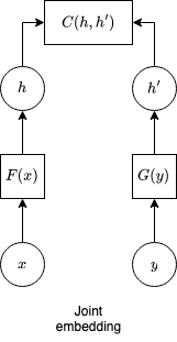
- In joint embedding, inputs can be both images.
- \(G(y)\) can be invariant to changes of luminosity, for example.
- This means we get multiple values of \(y\) with same \(h'\).
- Specific case: siamese nets, when \(F,G\) are identical
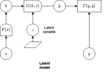
- General setup for latent variable: \(E(x, y, z)\) where \(z\) latent
- Find \(argmin_y min_z E(x, y, z)\)
- Can eliminate z replacing \(E\) with free energy: \(F_\beta(x, y) = - \frac{1}{\beta} \log \int_z e^{- \beta E(x, y, z)} dz\)
- When \(\beta=\infty\), this becomes \(F_\infty(x, y) = min_z E(x, y, z)\)
- Called free energy by physicists
- We use energy models when marginal probability in Gibbs-Boltzmann distribution is intractable
- We diminish our ambitions here! Use energy as fundamental underlying object.
- Where does energy come from?
- That’s where the free energy formula comes from.
- K-means as energy model
- Limiting the capacity of the latent variable \(z\)
- k-means solves this by setting \(z\) to be discrete
- Training EBM
- Give it an architecture/energy function \(F(x, y)\)
- For each datapoint \((x[i], y[i])\), tweak \(F\) so energy is as small as possible
- Then, we need the energy of other \((x[i], y')\) to be as large as possible
- Keep \(F\) smoothxs
- Two methods:
- Contrastive method: push down \(F(x[i], y[i])\), push up other points \(F(x[i], y')\)
- Regularized/Architectural methods: build \(F(x, y)\) so that volume of low energy regions is minimized through regularization
- Contrastive
- C1: push down energy of data points, push up everything else
- Max likelihood
- C2: push down energy of data points, push up chosen locations
- Max likelihood with MC/MMC/HMC
- Contrastive divergence
- Metric learning/Siamese nets
- Ratio matching
- Noise contrastive estimation
- Min probability flow
- Adversarial generation/GAM
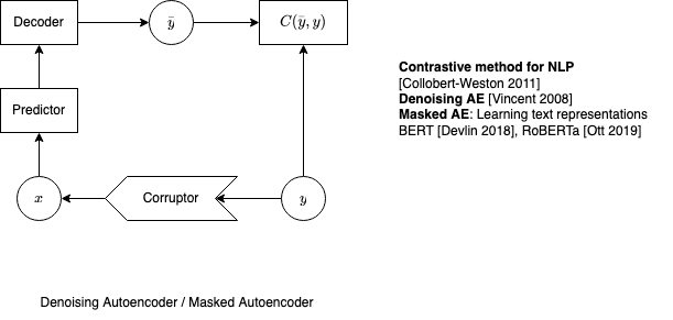
- C3: train a function that maps points off the data manifold to points on the data manifold:
- Denoising autoencoder
- Masked autoencoder (e.g. BERT)
- C1: push down energy of data points, push up everything else
- Regularized/Architectural
- A1: build the machine so the volume of low energy space is bounded:
- PCA
- K-means
- Gaussian mixture model
- Square ICA
- Normalizing flows
- A2: use a regularization term that measures the volume of space that has low energy:
- Sparse coding
- Sparse auto-encoder
- LISTA
- Variational auto-encoders
- Discretization/VQ/VQVAE
- A3: \(F(x, y)=C(y, G(x, y))\), make \(G(x, y)\) as “constant” as possible with respect to \(y\)
- Contracting auto-encoder
- Saturating auto-encoder
- A4: minimize the gradient and maximize the curvature around data points: score matching
- A1: build the machine so the volume of low energy space is bounded:
Why is max likelihood a contrastive method: we want to pick weights \(w\) to maximize
\[\begin{align*} p_w(y \vert x) &= \frac{e^{- \beta F_w(x, y)}}{\int_{y'}e^{- \beta F_w(x, y')}dy'} \\ \end{align*}\]Taking logs, this is same as to minimize:
\[\begin{align*} \mathcal{L}(x, y, w) &= F_w(x, y) + \frac{1}{\beta} \log \int_{y'}e^{- \beta F_w(x, y')}dy' \end{align*}\]Taking gradient w/ respect to \(w\):
\[\begin{align*} \frac{\partial}{\partial w}\mathcal{L}(x, y, w) &= \frac{\partial}{\partial w} F_w(x, y) + \frac{1}{\beta} \frac{\partial}{\partial w} \log \int_{y'}e^{- \beta F_w(x, y')}dy'\\ &= \frac{\partial}{\partial w} F_w(x, y) + \frac{1}{\beta} \frac{\frac{\partial}{\partial w} \int_{y'}e^{- \beta F_w(x, y')}dy'}{\int_{y'}e^{- \beta F_w(x, y')}dy'} \\ &= \frac{\partial}{\partial w} F_w(x, y) + \frac{1}{\beta} \frac{ \int_{y'}\frac{\partial}{\partial w}e^{- \beta F_w(x, y')}dy'}{\int_{y'}e^{- \beta F_w(x, y')}dy'} \\ &= \frac{\partial}{\partial w} F_w(x, y) - \frac{ \int_{y'}e^{- \beta F_w(x, y')}\frac{\partial}{\partial w}F_w(x, y')dy'}{\int_{y'}e^{- \beta F_w(x, y')}dy'} \\ &= \frac{\partial}{\partial w} F_w(x, y) - \int_{y'} p(y' \vert x) \frac{\partial}{\partial w}F_w(x, y')dy' \\ \end{align*}\]We can backpropagate through the left term.
Under the integral, if \(y'\) has high energy, \(p(y' \vert x)\) is low, and \(\frac{\partial}{\partial w}F_w(x, y')\) is not pushed up very much. If \(y'\) has low energy, \(p(y' \vert x)\) is high, \(\frac{\partial}{\partial w}F_w(x, y')\) is pushed up.
Issues
- Integral is most time intractable
- You can discretize the integral, but you still have to sum over all y. If \(y\) is in a discrete space, \(F\) is actually softmax.
- If the space is large, even discretized, it is too large.
- We can instead pick a single sample \(y'\).
- Back during WW2, during the Manhattan project, physicists invented the Monte-Carlo method, for a distribution that has only the energy, and not the distribution.
- MC/MCMC/HMC/CD: Draw a sample \(\hat{y}\) from \(F_w(y \vert x))\), and replace the integral with that sample.
- If you draw sufficiently many samples, get good approximation:
- If \(y\) space is very large, you will need a lot of samples
- Boltzmann machines, restricted Boltzmann machines - this is how they are trained
- MC, or MCMC methods for probabilistic graphical models - this is how they are trained
- \(\beta\) is to some extent arbitrary. You can pick value 1. For example, if you use softmax, you can rescale the previous layer so that \(\beta\) in the softmax becomes 1.
Gradient descent:
\[\begin{align*} w & \leftarrow w - \eta \frac{\partial}{\partial w}\mathcal{L}(x, y, w) \\ &= w - \eta \frac{\partial}{\partial w} F_w(x, y) + \eta \frac{\partial}{\partial w}F_w(x, \hat{y}) \end{align*}\]- First \(\eta\) term pushes down on the energy of samples
- Second \(\eta\) term pushes up on the energy of low-energy samples
Problems with this method:
- Large space of \(y\) requires many samples
- This method wants to push the bad \(y\)s to infinite energy
- Tell this to a statistician, they will murder you on the spot! It says the probabilistic approach does not function.
- Baesian statisticians have invented all sorts of things to prevent this from happening
- The loss must be regularized to keep the energy smooth
- But those are hacks, and you might as well use good hacks!
Instead of insisting that the energy is a log probability - just ensure that the energy of good points is lower than that of bad points.
Example cost functions:
- Simple: Bromley 1993:
- Pick non-matching \(\hat{y}\) by some method
- Push up \(F_w(x, \hat{y})\) but not more than \(m(y, \hat{y})\)
-
\([]^+\) is ReLU function
- Hinge pair loss: Altun 2003, Ranking loss: Weston 2010: I don’t care if \(F_w(x, y)\) is close to 0, I just want it less than \(F_w(x, \hat{y})\)
- Square-square loss: Chopra CVPR 2005, Hadsell CVPR 2006:
- Square ensures convexity, which helps convergence
- All possible outputs: Hinge loss
- Group losses: Neighborhood Component Analysis, Noise Contrastive Estimation (implicit infinite margin): Goldberger 2005, Gutmann 2010, …, Misra 2019, Chen 2020
- Contrastive joint embeddings

- Denoising or mask autoencoder
06L - Latent variable EBMs for structured prediction slides
- Recap of last lecture
- Group losses: Neighborhood Component Analysis, Noise Contrastive Estimation (implicit infinite margin): Goldberger 2005, Gutmann 2010, …, Misra 2019, Chen 2020
- Used with a batch that contains \(y\) and all \(\hat{y}_i\)
- If a single \(\hat{y}_i\) has low energy, and all other \(\hat{y}_j\) have high energy, gradient of weights will be pushed hard around \(\hat{y}_i\) but not other \(\hat{y}_j\)
- SSL for speech recognition: Wav2Vec2.0: Baevski et al. NeurIPS 2020, Xu et al. ArXiv:2010.11430, Github: PyTorch/fairseq
- Raw audio → ConvNet → Transformer
- Create foundational model trained on 960h speech with contrasting embedding of speech
- Transfer learning for 10m, 1h or 100h of labeled speech
- XLSR: multilingual speech recognition: Conneau arXiv:2006.13979
- Raw audio → ConvNet → Transformer
- GANs as contrastive energy models
- References
- J. Zhao, M. Mathieu, Y. LeCun: Energy-Based GANs (2017)
- M. Arjovsky et al: Wasserstein GAN (2017)
- Need to figure out how to pick samples whose energy to push up
- In GANs, push samples that have low energy, but are not part of training
- Will train a NN \(Gen(z)\) to generate the bad samples
- References

- Pick \(y, \hat{y}\). Backpropagate through \(Critic(y)\) to increase \(C(\hat{y},y)\).
- Backpropagate \(\hat{y}\) through both nets, but freeze \(Critic()\) and change weights only in \(Gen(z)\). This reduces energy of \(\hat{y}\)
- \(Gen(z)\) is trained to produce the negative samples
- Drop the critic to generate images
- GANs did not work very well originally
- Energy-Based GAN [Zhao 2016], Wasserstein GAN [Arjovsky 2017],… improved GANs by making energy function smooth. If you’re not careful, energy surface becomes canyon. You have to regularize the critic, and that’s essentially what Wasserstein GANs do.
- Optimization is finding a Nash equilibrium (a saddle point). With gradient descent, hard to find - get mode collapse, when critic does not give any useful gradients (and generator keeps producing same output)
- With original GANs, if you train long enough, you have collapse
- Wasserstein GANs are a way to deal with this. Though even with Wasserstein GANs, if you train long enough, you get mode collapse.
- Attempts to use critic as base for transfer learing have failed. Only generator can be used to generate data.
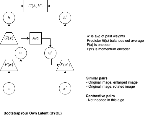
Non-Contrastive Methods for Joint Embedding
- Eliminates hard negative mining
- Siamese nets with slightly different weights
- Bootstrap Your Own Latent (BYOL), J-B Grill et al (2020), Deep Mind
- Use siamese networks
- But right network uses average of past weights of left network
- Idea is from MOCO - momentum embedded in these weights
- But MOCO largely outdated in last year or two
- Bootstrap Your Own Latent (BYOL), J-B Grill et al (2020), Deep Mind
- SwAV, Caron arXiv:2006.09882
- DeepCluster, Caron arXiv:1807.05520
- SimSiam: [Exploring Simple Siamese Representations)(https://arxiv.org/pdf/2011.10566.pdf), Chen et al, 2020
- Barlow Twins, Zbontar et al. ArXiv:2103.03230
- Use SwAV as foundational model for SEER, Goyal et al. ArXiv:2103.01988
Latent Variable Models in Practice
- Use latent variable when you can have multiple outputs for same input - or if output has some structure
- As you vary latent variable, prediction varies over all plausible outputs that correspond to input
- DETR: End-to-End Object Detection with Transformers, Carion et al (2020)
- ConvNet → Transformer
- ConvNet invariant to translation
- Transformer invariant to permutation (if input is permuted, so is output)
- Can do semantic segmentation with it
- ConvNet → Transformer
07L - PCA, AE, K-means, Gaussian mixture model, sparse coding, and intuitive VAE, slides
- Recap
- Faces have 50 degrees of freedom - suggest dimension of latent space
- Architectural models limit the dimension of the latent space
- PCA is an autoencoder with projection encoder, linear decoder.
- Energy: \(F_w(y) = \vert \vert y - Dec(Enc(y)) \vert \vert ^2 = \vert \vert y - w^Ty \vert \vert ^2\)
- Loss: \(L(y,w)=F_w(y)\)
- If using linear encoder (instead of projection), get PCA latent representation but up to affine transform (rotation+translation) in the latent space
- Auto-encoder
- Energy: \(F_w(y) = \vert \vert y - Dec(Enc(y)) \vert \vert ^2\)
- Loss: \(L(y,w)=F_w(y)\)
- k-Means
- Discrete latent-variable model with linear decoder
- Energy: \(E(y,z) = \vert \vert y - Dec(z) \vert \vert ^2 = \vert \vert y - wz \vert \vert ^2\)
- Free Energy: \(F(y) = \underset{z \in Z}{\min} E(y,z)\)
- Loss: \(L(y,w)=F_w(y)\)
- Latent vector \(z\) is constrained to be 1-hot vector \([..., 0, 1, 0, ...]\)
- \(wz\) selects one colum of \(w\)
- Free energy minimized around colums of \(w\)
- Algorithm:
- We’re given set of samples \(y\)
- Pick \(w\)
- Compute loss \(L(y, w)\) on set of samples \(y\)
- Change \(w\) in the direction of minimizing loss, either using gradient descent, or, in this case, direct computation.
- You don’t need contrastive learning, you don’t need to push on anything, b/c volume of latent variable is constrained - in this case, actually discrete.
- Don’t necessarily need a linear decoder for this to work.
- Gaussian Mixture Model
- Similar to k-means with soft marginalization over latent
- k-means use quadratic balls
- Gaussian mixture allows balls to take any shape within quadratic form - allow them to be elongated in some directions but not others
- Gaussian mixture can be “elongated along the data”. Thus, it can model the data with fewer samples.
- Energy: \(E(y, z) = (y-wz)^T (Mz) (y-wz)\)
- Here \((Mz)_{ij} = \sum_{k} M_{kij}z_k\)
- Free Energy: \(F(y) = - \frac{1}{\beta} \log \sum_{z \in Z} e^{\beta E(y,z)}\) (but LeCun says he’s missing a term - the mixture coefficients, that compute a weighted sum of the energies)
- Loss: \(L(y,w) = F_w(y)\) with normalization constraint on \(M\)
- Latent vector \(z\) is constrained to be 1-hot vector \([..., 0, 1, 0, ...]\)
- But marginalization makes it soft
- \(wz\) selects column of \(w\)
- Columns of \(w\) are centers of Gaussians
- Then, compute a distance, but distance is warped by a certain tensor \(M\), symmetric positive semi-definite, which is actually the universe covariance matrix of the Gaussians
- \(z\) being one-hot vector, it selects slice of matrix \(M\).
- Think of \(M\) as several slices of covariance matrices. \(z\) selects one of them.
- \(z\) selects the mean, then selects the covariance matrix
- Overall energy of Mixture is marginalization over \(z\).
- We’re not minimizing anymore, we’re marginalizing.
- You can set \(\beta\) to 1, it does not matter. Make a choice.
- How do you train it?
- Use EM (Expectation Maximization)
- You could use gradient descent, does not work very well. Gets you stuck to a local minimum.
- Will not explain EM.
- It’s an architectural model because you constrain the \(M\) matrix
- You have to guarantee that the covariance matrix has constant determinant.
- Similar to k-means with soft marginalization over latent
- Regularized Energy Based Models
- Instead of constraining the volume of the latent variable, have a regularization term that will constrain it
- Energy: \(E(x, y, z) = C(y, Dec(Pred(x),z)) + \lambda R(z)\)
- Examples of \(R(z)\):
- Effective dimension
- Quantization / discretization. Bayesians do this with Dirichlet allocation. Called LDA - Latent Dirichlet Analysis. Dirichlet can be pronounced in French, but he was German actually.
- L0 norm (# of non-zero components of a vector). Find \(z\) that I could use, such that \(z\) has minimum non-zero components. Will pay a price for each non-zero component. Problem: not a differential criterion. Hard to optimize. There are approximate methods, one is projection pursuit: find a component where you can project, to minimize cost. Then, find a 2nd component you can project, to still minimize cost, and so on.
- L1 norm with decoder normalization. Compute the sum of the absolute values of the components of \(z\). Minimize that. Called sparse coding. Compared to L0, it is a convex method. And it’s an approximation of L0 - it produces a sparse vector, eventually. L1 norm method is called sparse coding. Decoding is called sparse decoding.
- Maximize lateral inhibition / competition.
- Add noise to z while limiting its L2 norm (VAE)
- I forbid \(z\) to go outside a given sphere, but I add noise to \(z\) to make it a fuzzy value. LeCun applauds while speaking, to make the point that you have to focus on content while he adds noise.
- References
- K. Evtimova, Y. LeCun: Sparse Coding with Multi-layer Decoders using Variance Regularization (2022)
08L – Self-supervised learning and variational inference , slides
- Review of GANs as constrastive energy-based models (EBMs)