Top | Notations | Bibliography
What is Reinforcement Learning?
In machine learning, there are three types of learning tasks:
- Supervised learning (given a set of annotated input, learn to predict output)
- Unsupervised learning (discover a good representation of the input)
- Reinforcement learning (learn to select actions that maximize reward)
In supervised & unsupervised learning, the object being learned is data - for example text, speech, images. In reinforcement learning (RL), what is learned are processes, using a reward function to determie the optimal actions.
The CartPole example
In this example, a pole is balanced on top of a cart. The environment is two-dimensional. The cart needs to be moved left or right to balance the pole.
- The objective is to keep the pole upright
- The state is represented by (cart position, cart speed, pole angle, pole angular speed)
- The action is to move the cart a unit of distance to the left, or a unit of distance to the right
- The reward is \(+1\) for each step the pole remains upright (i.e., does not tip for more than a fixed angle)
Over multiple learning episodes, the agent learns to balance the pole. This is a simple example when the neural network (NN) training does not require a GPU, and learning can be reasonably achieved within around 200 episodes. The algorithm used is REINFORCE.
Formulation of the problem
In reinforcement learning (RL), an agent reads state \(s_t\) from the environment, acts with action \(a_t\), and moves the environment to state \(s_{t+1}\) with reward \(r_{t+1} \in \mathbb{R}\). The cycle then continues, creating a feedback loop:

The agent-environment interation in a Markov Decision Process
The process can end after a finite number of steps \(T\), or can continue indefinitely. The agent’s goal is to learn a policy \(\pi(a_t \vert s_t)\) that defines the distribution of actions \(a_t\) conditioned by state \(s_t\), with the goal of maximizing the sum of all rewards for the next steps \(r_{t+1} + r_{t+2} + ...\).
If we denote \(\mathcal{S}, \mathcal{A}\) the set of states and actions, then the policy \(\pi\) is a conditional distribution \(\pi(a_t \vert s_t)\) of actions \(a_t \in \mathcal{A}\) conditioned by states \(s_t \in \mathcal{S}\).
The objective of RL problems is to maximize the sum of future rewards, learning a good policy \(\pi\), through trial and error, using the size of rewards to reinforce good actions.
Markov Decision Process
The states \(s_{t+1}\), in practice, can only be estimated, stochastically, up to a measurement error:
\[\begin{equation} s_{t+1} \sim p(s_{t+1} \vert s_0,a_0,s_1,a_1,...,s_t,a_t) \end{equation}\]At each step, the state $s_{t+1}$ is sampled from a probability distribution \(P\) conditoned on past states and actions. To simplify things, we assume that all the information from past states and actions is subsumed into \((s_t, a_t)\), turning the process into a Markov Decision Process (MDP):
\[\begin{equation} \label{eq:state_transition_dist} s_{t+1} \sim p(s_{t+1} \vert s_t,a_t) \end{equation}\]This formulation is still flexible enough to provide good models. If the process is not Markov, and \(s_{t+1}\) depends on additional information than \((s_t,a_t)\), the state space can often be extended to turn the process into an MDP. The CartPole process, for example, is a Markov process, because the next state is an exact function of the current state and action.
The reward \(r_{t+1} \in \mathbb{R}\) is assigned for transitioning from state \(s_t\) through action \(a_t\) to state \(s_{t+1}\). We can extend the probability distribution to include rewards:
\[\begin{align} s_{t+1}, r_{t+1} \sim p(s_{t+1}, r_{t+1} \vert s_t,a_t) \end{align}\]This is a slightly more general formulation where the rewards are seen as a conditional distribution over \(s_t, a_t\) unrelated to the next state \(s_{t+1}\).
In an MDP, \(p(s_{t+1}, r_{t+1} \vert s_t,a_t)\) represents the state transition distribution.
To simplify notations, we denote \(s'\) the successor state of a state \(s\) when applying action \(a\). The state transition distribution then can be written as \(p(s',r \vert s,a)\).
A Markov Decision Process (MDP) consists, in general, of
- A set of states \(\mathcal{S}\) and actions \(\mathcal{A}\)
- Probability measures \(ds\) and \(da\) on \(\mathcal{S}\) and \(\mathcal{A}\)
- A distribution of the initial state \(p(s)\)
- A state transition probability distribution \(p(s', r \vert s, a)\) representing the probability of arriving to state \((s', r)\) fron \(s\) when applying action \(a\)
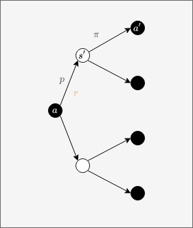
Here is an example of a finite MDP (source):
- The yellow nodes are states \(s\)
- The blue diamonds are actions \(a\), with stochastic outcomes and rewards labeled with \(p(s' , r \vert s, a)\)
- The ribbons (and bombs) are the rewards \(r\)
 Workday Model (source)
The state transition model
The state transition distribution \(p(s', r \vert s, a)\) satisfies
\[\begin{align*} \int_{s' \in \mathcal S} \int_{r \in \mathbb{R}} p(s', r \vert s, a) drds'= 1 \textrm{ for all } s \in \mathcal{S} \textrm{ and } a \in \mathcal{A} \end{align*}\]We define a partial probability \(\begin{align} p(s' \vert s, a) = Pr\big(s_{t+1} = s' \vert s_t = s, a_t = a\big) = \int_{r \in \mathbb{R}} p(s', r \vert s, a) dr \end{align}\)
and call this the state transition model of the MDP.
In the Workday Model example, \(p(s' \vert s, a)\) is known for all states \(s\) and actions \(a\). In this case, we say that the model is known. Agents do not always have direct access to the model \(p(s' \vert s, a)\), but they may, however, sample it.
Expected reward functions
We can compute an expected reward for a state-action pair as a function \(r \, : \, \mathcal{S} \times \mathcal{A} \rightarrow \mathbb{R}\) given by
\[\begin{align} r(s, a) = \mathbb{E}\big[r_{t+1} \vert s_t = s, a_t = a\big] = \int_{r \in \mathbb{R}} r \int_{s' \in \mathcal{S}} p(s', r \vert s, a) ds' dr \end{align}\]and an expected reward for a state-action-state as a function \(r \, : \, \mathcal{S} \times \mathcal{A} \times \mathcal{S} \rightarrow \mathbb{R}\) given by
\[\begin{align} r(s, a, s') = \mathbb{E}\big[r_{t+1} \vert s_t = s, a_t = a, s_{t+1} = s'\big] = \int_{r \in \mathbb{R}} r \, \frac{p(s', r \vert s, a)}{p(s' \vert s, a)} dr \end{align}\]In most models, we often define our own choice of reward functions. For example, in the Workday Model the reward is a function of state-action-states. Some papers assume that the reward is a function of the states-actions (e.g., the S. Levine tutorial), in which case the state-action-state reward can be derived1.
State-Action Trajectories
A sequence of states and actions defines a possibly infinite state-action trajectory
\[\begin{equation} \label{eq:tau} \tau = (s_0, a_0, s_{1}, a_{1}, ... , s_{T-1}, a_{T-1}, s_T) \end{equation}\]The trajectory probability with a given policy \(\pi\), under the Markov assumption, is given by
\[\begin{equation} \label{eq:taudist} p_\pi(\tau) = p(s_0) \prod_{t=0}^{T-1} \pi(a_t \vert s_t) \prod_{t=0}^{T-1} p(s_{t+1} \vert s_t, a_t) \end{equation}\]State-Action-Rewards Trajectories
If we pick rewards along a trajectory \(\tau\), we get a state-action-reward trajectory \(\begin{align} \overline{\tau} = (s_0, a_0, r_1, s_1, a_1, r_2, ..., s_{T-1}, a_{T-1}, r_T, s_T) \end{align}\) with probability \(\begin{align} p_\pi(\overline{\tau}) & = p(s_0) \prod_{t=0}^{T-1} \pi(a_t \vert s_t) \prod_{t=0}^{T-1} p(s_{t+1},r_{t+1} \vert s_t, a_t) \end{align}\)
Each state-action-reward trajectory \(\overline{\tau}\) has an underlying state-action trajectory \(\tau\) obtained by forgetting the rewards.
Truncated trajectories
The formulas in this section are necessary for later deriving the Bellman equations. Trajectories can be truncated to \(\tau_{>s_t} = (a_t, s_{t+1}, ... , s_T)\) and \(\tau_{>a_t} = (s_{t+1}, a_{t+1}, ... , s_T)\). The probabilities of the truncated trajectories are:
\[\begin{align} \label{eq:taudists} p_\pi(\tau_{>s_t} \vert s_t) = \prod_{t'=t}^{T-1} \pi(a_{t'} \vert s_{t'}) \prod_{t'=t}^{T-1} p(s_{t'+1} \vert s_{t'}, a_{t'}) \\ \end{align}\] \[\begin{align} \label{eq:taudistsa} p_\pi(\tau_{>a_t} \vert s_t, a_t) = \prod_{t'=t+1}^{T-1} \pi(a_{t'} \vert s_{t'}) \prod_{t'=t}^{T-1} p(s_{t'+1} \vert s_{t'}, a_{t'}) \\ \end{align}\]Trajectories can also be truncated down: \(\tau_{\le a_t} = (s_0, a_0, ... , s_{t}, a_{t})\). If \(\overline{\tau}\) is a state-action-reward trajectory, it can also be truncated up \(\overline{\tau}_{>s_t}, \overline{\tau}_{>a_t}\) or down \(\overline{\tau}_{\le a_t}\), with probability formulas similar to the ones above, replacing \(p(s_{t'+1}|s_{t'},a_{t'})\) with \(p(s_{t'+1}, r_{t'+1}|s_{t'},a_{t'})\).
Rewards and the Return of a Trajectory
In RL problems, action \(a_t\) is picked not just to maximize next reward $r_{t+1}$, but the sum of all future rewards \(r_{t+1} + r_{t+2} + ...\). If the number of steps is infinite, even if all rewards are bounded, the sum may not converge. It is convenient, then, to discount rewards by a factor \(0 \le \gamma \le 1\), which is \(\lt 1\) if the number of steps is infinite, and define the return of a state-action-reward trajectory \(\overline{\tau}\) as
\[\begin{align} \overline{\tau} = (s_0, a_0, r_1, ... , s_{T-1}, a_{T-1}, r_T, s_T) \end{align}\]as
\[\begin{equation} \label{eq:traj_return} r(\overline{\tau}) = r_{1} + {\gamma}r_{2} + {\gamma^2}r_{3} + ... + {\gamma^{T-1}}r_{T} \end{equation}\]The larger the discount factor \(\gamma\), the larger the effect of later steps. The smaller the discount factor, the bigger weight is given to actions taken for the immediate next steps.
In what follows, we assume that rewards are bounded by \(-M \le r_t \le M\) for all \(t\), and \(\gamma \lt 1\). When the number of steps is infinite, then \(r(\overline{\tau})\) is uniformly convergent with respect to all choices of infinite trajectories:
\[\begin{equation} r(\overline{\tau}) = \sum_{t=1}^{\infty} \gamma^{t-1}r_t \end{equation}\]The Agent Objective and the Value Functions
Recall that we denote \(\overline{\tau}\) for an state-action-reward trajectory, and \(\tau\) for a state-action trajectory.
When trajectories \(\overline{\tau}\) are sampled according to a policy \(\pi\), we would like to define the agent objective as the expected value of the return function of infinite trajectories \(\overline{\tau}\), sampled over the policy distribution \(p_\pi(\tau)\) defined by (\(\ref{eq:taudist}\)):
\[\begin{equation} "J_\pi = \mathbb{E} \big[\big( \sum_{t=1}^{\infty} \gamma^{t-1}r_t \big) \, \vert \, s_0, a_0, r_1, s_1, a_1, r_1, ... \sim \pi\big] " \end{equation}\]We place this between double quotes, because, mathematically, these entities are not yet well defined. The probability of an infinite trajectory is not defined. We can work around that, however, using the fact that the discounted reward series
\[\begin{align} \sum_{t=1}^{\infty} \gamma^{t-1}r_t \end{align}\]is uniformly convergent for all trajectories. Thus, we can define the agent objective as
\[\begin{equation} \label{eq:objective} J_\pi = \underset{T \rightarrow \infty}{lim} \mathbb{E}_{\tau \sim \pi}[\sum_{t=0}^{T-1} \gamma^{t} r(s_t, a_t)] \end{equation}\]The goal of the agent is to find a policy \(\pi\) that maximizes the objective \(J_\pi\). If we fix the initial state \(s\), or the pair \((s, a)\) of initial state and initial action, we define the state-value function
\[\begin{equation} \label{eq:value_state} V_\pi(s) = \underset{T \rightarrow \infty}{lim} \mathbb{E}_{s_0=s, \tau \sim \pi}[\sum_{t=0}^{T-1} \gamma^{t} r(s_t, a_t)] \end{equation}\]and the action-value function
\[\begin{equation} \label{eq:value_state_action} Q_\pi(s, a) = \underset{T \rightarrow \infty}{lim} \mathbb{E}_{s_0=s, a_0=a, \tau \sim \pi}[\sum_{t=0}^{T-1} \gamma^{t} r(s_t, a_t)] \end{equation}\]\(V_\pi(s)\) evaluates how good the state \(s\) is, and \(Q_\pi(s, a)\) evaluates how good action \(a\) is in state \(s\), according to the policy \(\pi\). \(V\) stands for value, and \(Q\) for quality.
Expressing value functions as integrals
Recall that \(\tau\) denotes a trajectory \(s_0, a_0, ...\). We denote for convenience \(\tau_{>s_t}\) for the truncated data set \(a_t, s_{t+1}, ...\) and \(\tau_{>a_t}\) for the truncated trajectory \(s_{t+1}, a_{t+1}, ...\)
Applying the definition of density to objective \(J_\pi\), the state-value \(V_\pi(s)\) and the action-value \(Q_\pi(s, a)\) functions, we get:
\[\begin{align} J_\pi & = \underset{T \rightarrow \infty}{lim} \sum_{t=0}^{T-1} \int_{\tau_{\le a_t} = s_0, a_0, ... , a_t} \gamma^{t} r(s_t, a_t) p_\pi(s_t, a_t \vert \tau) d\tau_{\le a_t} \hspace{1cm} \\ V_\pi(s_0) & = \underset{T \rightarrow \infty}{lim} \sum_{t=0}^{T-1}\int_{\tau_{>s_0 \le a_t} = a_0, s_1, a_1, ... , a_t} \gamma^{t} r(s_t, a_t) p_\pi(s_t, a_t \vert \tau_{>s_0}) d\tau_{>s_0 \le a_t} \hspace{1cm} & \\ Q_\pi(s_0, a_0) & = \underset{T \rightarrow \infty}{lim} \sum_{t=0}^{T-1} \int_{\tau_{>a_0 \le a_t} = s_1, a_1, ..., a_t} \gamma^{t} r(s_t, a_t) p_\pi(s_t, a_t \vert \tau_{>a_0}) d\tau_{>a_0 \le a_t} \hspace{1cm} & \\ & = r(s_0,a_0) + \underset{T \rightarrow \infty}{lim} \sum_{t=1}^{T-1} \int_{\tau_{>a_0 \le a_t} = s_1, a_1, ..., a_t} \gamma^{t} r(s_t, a_t) p_\pi(s_t, a_t \vert \tau_{>a_0}) d\tau_{>a_0 \le a_t} \hspace{1cm} & \\ \end{align}\]The Bellman Expectation Equations
The objective \(J_\pi\), the state-value \(V_\pi(s)\) and the action-value \(Q_\pi(s, a)\) functions are interrelated. To show that, we express them in terms of the trajectory distribution \(p_\pi(\tau)\) of (\(\ref{eq:taudist}\)).
\[\begin{align} J_\pi & = \underset{T \rightarrow \infty}{lim} \sum_{t=0}^{T-1} \int_{\tau_{\le a_t} = s_0, a_0, ... , a_t} \gamma^{t} r(s_t, a_t) p_\pi(s_t, a_t \vert \tau) d\tau_{\le a_t} \hspace{1cm} \\ & = \underset{T \rightarrow \infty}{lim} \sum_{t=0}^{T-1} \int_{\tau_{\le a_t} = s_0, a_0, ... , a_t} \gamma^{t} r(s_t, a_t) \prod_{t'=0}^{t-1} \pi(a_{t'} \vert s_{t'}) \prod_{t'=0}^{t-1} p(s_{t'+1} \vert s_{t'}, a_{t'}) d\tau_{\le a_t} \hspace{1cm} & (expand \, p_\pi(s_t, a_t \vert \tau)) \\ & = \underset{T \rightarrow \infty}{lim} \sum_{t=0}^{T-1} \int_{s_0} \big( \int_{\tau_{>s_0 \le a_t} = (a_0, s_1, ..., a_t)} \gamma^{t} r(s_t, a_t) \prod_{t'=0}^{t-1} \pi(a_{t'} \vert s_{t'}) \prod_{t'=0}^{t-1} p(s_{t'+1} \vert s_{t'}, a_{t'}) d\tau_{>s_0\le a_t} \big) p(s_0)ds_0 \hspace{1cm} & (Fubini \, for \, d\tau_{\le a_t} = d\tau_{>s_0\le a_t} ds_0) \\ & = \int_{s_0} \big( \underset{T \rightarrow \infty}{lim} \sum_{t=0}^{T-1} \int_{\tau_{>s_0 \le a_t} = (a_0, s_1, ..., a_t)} \gamma^{t} r(s_t, a_t) \prod_{t'=0}^{t-1} \pi(a_{t'} \vert s_{t'}) \prod_{t'=0}^{t-1} p(s_{t'+1} \vert s_{t'}, a_{t'}) d\tau_{>s_0\le a_t} \big) p(s_0) ds_0 \hspace{1cm} & (uniform \, convergence) \\ & = \int_{s} V_\pi(s) p(s) ds & (definition \, of \, V_\pi(s)) \\ \end{align}\]This says that \(J_\pi\) is the expected value of \(V_\pi(s)\) over all states \(s\). We also have:
\[\begin{align} V_\pi(s_0) & = \underset{T \rightarrow \infty}{lim} \sum_{t=0}^{T-1}\int_{\tau_{>s_0 \le a_t} = a_0, s_1, a_1, ... , a_t} \gamma^{t} r(s_t, a_t) p_\pi(s_t, a_t \vert \tau_{>s_0}) d\tau_{>s_0 \le a_t} \hspace{1cm} & (definition \, of \, expectation) \\ & = \underset{T \rightarrow \infty}{lim} \sum_{t=0}^{T-1} \int_{a_0} \pi(a_0 \vert s_0) \big( \int_{\tau_{>a_0 \le a_t} = s_1, a_1, ..., a_t} \gamma^{t} r(s_t, a_t) p_\pi(s_t, a_t \vert \tau_{>s_0}) d\tau_{>a_0 \le a_t} \big) da_0 \hspace{1cm} & (Fubini \, for \, d \tau_{>s_0} = d \tau_{>a_0 \le a_t} da_0) \\ & = \int_{a_0} \pi(a_0 \vert s_0) \big( \underset{T \rightarrow \infty}{lim} \sum_{t=0}^{T-1} \int_{\tau_{>a_0 \le a_t} = s_1, a_1, ..., a_t} \gamma^{t} r(s_t, a_t) p_\pi(s_t, a_t \vert \tau_{>s_0}) d\tau_{>a_0 \le a_t} \big) da_0 \hspace{1cm} & (uniform \, convergence) \\ & = \int_{a_0} \pi(a_0 \vert s_0) Q_\pi(s_0, a_0) da_0 \hspace{1cm} & (definition \, of \, Q_\pi(s_0, a_0)) \\ \end{align}\]Relabeled, this says that \(\begin{align} \label{eq:vq_bellman} V_\pi(s) = \int_a \pi(a \vert s) Q_\pi(s, a) da \end{align}\)
which means that \(V_\pi(s)\) is the expected value of \(Q_\pi(s, a)\) over all actions \(a\) in state \(s\). And we can also express \(Q_\pi(s, a)\) in terms of \(V_\pi\):
\[\begin{align} Q_\pi(s_0, a_0) & = r(s_0,a_0) + \underset{T \rightarrow \infty}{lim} \sum_{t=1}^{T-1} \int_{\tau_{>a_0 \le a_t} = s_1, a_1, ..., a_t} \gamma^{t} r(s_t, a_t) p_\pi(s_t, a_t \vert \tau_{>a_0}) d\tau_{>a_0 \le a_t} \hspace{1cm} & (as \, shown \, before) \\ & = r(s_0, a_0) + \gamma \underset{T \rightarrow \infty}{lim} \sum_{t=1}^{T-1} \int_{\tau_{>a_0 \le a_t} = s_1, a_1, ..., a_t} \gamma^{t-1} r(s_t, a_t) \prod_{t'=1}^{t-1} \pi(a_{t'} \vert s_{t'}) \prod_{t'=0}^{t-1} p(s_{t'+1} \vert s_{t'}, a_{t'}) d\tau_{>a_0 \le a_t} \hspace{1cm} & (definition \, of \, p_\pi(\tau_{>a_0 \le a_t})) \\ & = r(s_0, a_0) + \gamma \underset{T \rightarrow \infty}{lim} \sum_{t=1}^{T-1} \int_{\tau_{>a_0 \le a_t} = s_1, a_1, ..., a_t} p(s_{1} \vert s_0, a_0) \gamma^{t-1} r(s_t, a_t) \prod_{t'=1}^{t-1} \pi(a_{t'} \vert s_{t'}) \prod_{t'=1}^{t-1} p(s_{t'+1} \vert s_{t'}, a_{t'}) d\tau_{>a_0 \le a_t} \hspace{1cm} & (bring \, p(s_1 \vert s_0,a_0) \, out \, of \, \prod_{t'=0}^{t-1}) \\ & = r(s_0, a_0) + \gamma \underset{T \rightarrow \infty}{lim} \sum_{t=1}^{T-1} \int_{\tau_{>a_0 \le a_t} = s_1, a_1, ..., a_t} p(s_{1} \vert s_0, a_0) \gamma^{t-1} r(s_t, a_t) p_\pi(s_t, a_t \vert \tau_{>a_0 \le a_t}) d\tau_{>a_0 \le a_t} \hspace{1cm} & (replace \, with \, p_\pi(s_t, a_t \vert \tau_{>a_0 \le a_t})) \\ & = r(s_0, a_0) + \gamma \int_{s_1} p(s_{1} \vert s_0, a_0) V_\pi(s_1) ds_1 \hspace{1cm} & (definition \, of \, V_\pi(s_1) \, for \, T-1) \\ & = r(s_0, a_0) + \gamma \int_{s_1, a_1} \pi(a_1 \vert s_1) p(s_{1} \vert s_0, a_0) Q_\pi(s_1, a_1) ds_1 da_1 \hspace{1cm} & (V_\pi(s_1) \, as \, expected \, value \, of \, Q_\pi(s_1, a_1) \, over \, a_1) \\ \end{align}\]Relabeling notations, we get:
\[\begin{align} \label{eq:q_bellman} Q_\pi(s, a) & = r(s, a) + \gamma \int_{s',a'} \pi(a' \vert s') p(s' \vert s, a) Q_\pi(s',a') ds'da' \\ \end{align}\]The equations (\ref{eq:v_bellman}), (\ref{eq:q_bellman}) are the Bellman expectation equations for \(J_\pi\) and \(Q_\pi(s, a)\). Plugging back into the equation for \(V_\pi(s)\) we get
\[\begin{align} V_\pi(s) & = \int_a \pi(a \vert s) Q_\pi(s, a) da & \\ & = \int_a \pi(a \vert s) \big( r(s, a) + \gamma \int_{s',a'} p(s' \vert s, a) Q_\pi(s',a') ds'da'\big)da & (expand \, Q_\pi(s, a))\\ & = \int_a \pi(a \vert s) \big( r(s, a) + \gamma \int_{s'} p(s' \vert s, a) \big( \int_{a'} Q_\pi(s',a') da' \big) ds'\big)da & (Fubini \, for \, da'ds')\\ & = \int_a \pi(a \vert s) \big( r(s, a) + \gamma \int_{s'} p(s' \vert s, a) V_\pi(s') ds'\big)da & (regroup \, V_\pi(s')) \\ \end{align}\]This gives us the Bellman expectation equation for \(V_\pi(s)\): \(\begin{align} \label{eq:v_bellman} V_\pi(s) = \int_a \pi(a \vert s) \big( r(s, a) + \gamma \int_{s'} p(s' \vert s, a) V_\pi(s') ds'\big) da \\ \end{align}\)
Backup diagrams
The Bellman equations in this section were expressed in terms of state-action reward expectations \(r(s, a)\). We can express the same Bellman equations in terms of state-action-state reward expectations \(r(s, a, s')\), for example: \(\begin{align} V_\pi(s) = \int_{a, s'} \pi(a \vert s) \big( r(s, a, s') + \gamma p(s' \vert s, a) V_\pi(s') \big) ds' da \\ \end{align}\)
This can be visualized though the following backup diagram, where states are represented by white circles, and actions by black circles, state values \(V_\pi(s)\) being represented as the expected value (over \(\pi(a \vert s)\)) of the expected rewards \(r(s, a, s')\) plus discounted values \(\gamma V_\pi(s')\) (over \(p(s' \vert s, a)\)):

Backup diagram for state-action-state Bellman equation
We can express the Bellman equation for state-action values in terms of state-action-state reward expectations \(r(s, a, s')\) as follows: \(\begin{align} Q_\pi(s, a) & = \int_{s'} r(s, a, s') ds' + \gamma \int_{s',a'} \pi(a' \vert s') p(s' \vert s, a) Q_\pi(s',a') ds'da' \end{align}\)
This can be visualized on the following backup diagram:
Backup diagram for action-state-action Bellman equation
Optimal policies
The goal of RL is to find policies \(\pi\) that maximize the objective \(J_\pi\).
Policies have a partial order \(\pi_1 \le \pi_2\) defined by \(V_{\pi_1}(s) \le V_{\pi_2}(s)\) for all states \(s\) and actions \(a\). From the Bellman expectation equation \(\begin{align} Q_\pi(s, a) & = r(s, a) + \gamma \int_{s'} p(s' \vert s, a) V_\pi(s') ds' \end{align}\) we see that \(\pi_1 \le \pi_2\) implies \(Q_{\pi_1}(s, a) \le Q_{\pi_2}(s, a)\) for all states \(s\) and actions \(a\). (But if \(Q_{\pi_1}(s, a) \le Q_{\pi_2}(s, a)\) for all states \(s\) and actions \(a\), it is not necessarily true that \(\pi_1 \le \pi_2\), because the Bellman equation that expresses \(V\) in terms of \(Q\) involves not just the model \(p\) but also the policies \(\pi_1, \pi_2\)). And from the Bellman expectation equation \(\begin{align} J_\pi & = \int_{s} V_\pi(s) p(s) ds \end{align}\) we see that \(\pi_1 \le \pi_2\) implies \(J_{\pi_1} \le J_{\pi_2}\).
TO DO: Fix this below:
We attempt to construct a maximal policy as follows: for all states \(s\) and actions \(a\), define \(\begin{align} Q_\star(s, a) & = \underset{\pi}{sup} \, Q_\pi(s, a) \\ V_\star(s) & = \underset{\pi}{sup} \, V_\pi(s) \\ \end{align}\)
Since rewards are bounded, \(Q_\pi(s, a), V_\pi(a)\) are uniformly bounded for all \(a, \pi\), and \(Q_\star(s, a), V_\star(a)\) are well defined as \(sup\) of a bounded set of real numbers.
Pick \(\epsilon > 0\). Define a deterministic policy \(\pi_{\epsilon\star}\) that picks, in any state \(s\), an action \(a\) such that there exists a policy \(\pi_{\epsilon, s, a}\) satisfying
\[\begin{align} Q_{\pi_{\epsilon,s,a}}(s, a) \gt Q_\star(s, a) - \epsilon \end{align}\]This is possible to do because policies can be defined state by state. Then, we claim that \(\begin{align} Q_{\pi_{\epsilon\star}}(s, a) \gt Q_\star(s, a) - \epsilon \end{align}\) for all states \(s\) and actions \(a\).
Then, using the Bellman equation \(\begin{align} V_\pi(s) = \int_a \pi(a \vert s) Q_\pi(s, a) da \end{align}\) it is immediate that \(V_{\pi_{\epsilon\star}}(s) \gt \underset{a \in \mathcal{A}}{sup} Q_\star(s, a) - \epsilon\) for all \(\epsilon \gt 0\), so \(V_\star(s) \ge \underset{a \in \mathcal{A}}{sup} \, Q_\star(s, a)\). The inequality in the opposite direction \(V_\star(s) \le \underset{a \in \mathcal{A}}{sup} \, Q_\star(s, a)\) is obvious, so \(V_\star(s) = \underset{a \in \mathcal{A}}{sup} \, Q_\star(s, a)\). It is then straightforward to derive the entire set of equations below:
\[\begin{align} V_\star(s) & = \underset{a \in \mathcal{A}}{sup} \, Q_\star(s, a) \\ & = \underset{a \in \mathcal{A}}{sup} \big( r(s, a) + \gamma \int_{s'} p(s' \vert s, a) V_\star(s') ds'\big) \\ Q_\star(s, a) & = r(s, a) + \gamma \int_{s'} p(s' \vert s, a) \, V_\star(s') ds' \\ & = r(s, a) + \gamma \int_{s'} p(s' \vert s, a) \, \underset{a' \in \mathcal{A}}{sup} \, Q_\star(s',a') ds' \\ \end{align}\]These are called the Bellman optimality equations. For finite \(\mathcal{A}\), we have effectively constructed a maximal policy \(\pi_\star\), picking in state \(s\) the greedy action \(a\) that maximizes \(Q_\star(s, a)\) - while for infinite \(\mathcal{A}\), such a maximal policy may not exist, but can be uniformly approximated, for any \(\epsilon \gt 0\), by policies \(\pi_{\epsilon\star}\) such that \(Q_{\pi_{\epsilon\star}}(s, a) \gt Q_\star(s, a) - \epsilon\) and \(V_{\pi_{\epsilon\star}}(s) \gt V_\star(s) - \epsilon\) for all states \(s\) and actions \(a\).
Deep learning RL algorithms
Deep learning algorithms for RL problems can be classified as:
- Value based (algorithms learning value functions \(V_\pi(s)\) or \(Q_\pi(s, a\)), then deriving the policy \(\pi\))
- Policy based (algorithms learning the policy \(\pi\) directly)
- Model based (algorithms that know the environment dynamics \(p(s' \vert s, a)\), or learn it.
- Or combinations thereof.
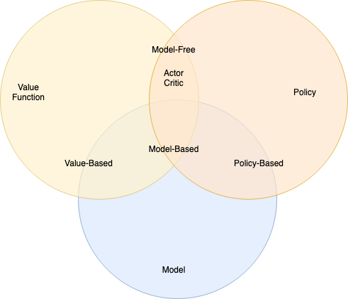
Algorithm Types (source)
The taxonomy below is from Foundations of Deep RL. See Sec. 1.4 in there for a more in depth discussion.
Value based algorithms
This class of algorithms learn the action-value functions \(Q_\pi(s, a)\). A policy \(\pi(a \vert s)\) could be picked, for example, to maximizes the action-value \(Q_\pi(s, a)\) in all states \(s\). It is less common to lear \(V_\pi(s)\) and infer the policy \(\pi\).
Example value based algorithms:
- Q-Learning
- SARSA
- Deep Q Networks (DQN)
- Variants of DQN: Double DQN, DQN with Prioritized Experience Replay (PER)
In the algorithms above, the set of states \(\mathcal{S}\) and actions \(\mathcal{A}\) must be finite. More recently, value based algorithms like QT-OPT have become available and can be applied to continuous action spaces \(\mathcal{A}\).
This class of algorithms are more sample efficient. They work well if \(Q_\pi(s, a)\) can be maximized without having to look ahead many action steps.
Policy based algorithms
These algorithms learn a policy \(\pi\) that maximizes the agent objective \(J_\pi\). Example algorithm:
- REINFORCE
In this class of algorithms, the space of actions \(\mathcal{A}\) can be either continuous or discrete. The disadvantage is that these algorithms have high variance and are sample inefficient.
Model based algorithms
These algorithms either know the environment dynamics \(p(s' \vert s, a)\), or learn it.
- Monte Carlo Tree Search (MCTS) is used when the space of states \(\mathcal{S}\) and actions \(\mathcal{A}\) are finite, and the transition functions \(p(s' \vert s, a)\) are known. In the past, MCTS was used for board games (Chess, Go).
- Linear Quadratic Regulators (iLQR), Model Predictve Control (MPC) involve learning \(p(s' \vert s, a)\).
Models are often unavailable, or can’t be learned. If they are, however, and if the number of states and actions is small, then model-based algorithms are an order of magnitude more efficient than value or policiy based algorithms.
Model-based algorithms, effectively, simulate the environment. If the estimation errors are small, the algorithm learned in simulation will work well when run in the actual environment. However, the estimation errors can compound quickly over several steps of actions.
Combined algoritms
- Actor-Critic methods use value and policy based methods. The policy (the ‘actor’) is learned using feedback from a learned action-value function (the ‘critic’).
- AphaGo, AlphaZero use a combination of supervised learning, RL model, value and policy based algorithms, and self-play.
1: Each MDP \((\mathcal{S}, \mathcal{A}, p(s_0), p(s',r \vert s, a))\) is equivalent to an MDP \((\mathcal{S}, \mathcal{A}, p(s_0), p(s', \rho \vert s, a))\) where \(\rho\) is induced by a function also denoted \(\rho \, : \, \mathcal{S} \times \mathcal{A} \rightarrow \mathbb{R}\) as \(p(\rho \vert s, a) = \delta_{\rho(s, a)}\) where \(\delta_{\rho(s, a)}\) is the Dirac probability with value 1 for \(\rho(s, a)\) and 0. See Equivalent Markov Decision Processes.