Top | Notations | Bibliography
Introduction
The sets of states \(\mathcal{S}\) and actions \(\mathcal{A}\) are assumed to be finite.
We have defined a partial order on policies, saying that \(\pi_1 \le \pi_2\) when \(Q_{\pi_1}(s, a) \le Q_{\pi_2}(s, a)\) for all states \(s\) and actions \(a\). From the Bellman expectation equations
\[\begin{align} V_\pi(s) & = \int_a \pi(a \vert s) Q_\pi(s, a) da \\ Q_\pi(s, a) & = r(s, a) + \gamma \int_{s'} p(s' \vert s, a) V_\pi(s') ds' \\ \end{align}\]we notice that \(\pi_1 \le \pi_2\) if and only if \(V_{\pi_1}(s) \le V_{\pi_2}(s)\) for all states \(s\).
The idea in value learning algorithms is to look for an optimal policy \(\pi\) that maximizes the action-value function \(Q_\pi(s, a)\) for all states \(s\) and actions \(a\).
The process is iterative. We start with policy \(\pi_1\), estimate \(Q_{\pi_1}(s, a)\) or \(V_{\pi_1}(s)\) for some or all states \(s\) and actions \(a\), find a more optimal policy \(\pi_2 \gt \pi_1\), and iterate the process \(\begin{align} \pi_1 \lt \pi_2 \lt ... \lt \pi_n \end{align}\)
until either we find the optimal policy \(\pi\) (which is possible to do in case the number of states and actions is small), or a sufficiently good approximation of the optimal policy \(\pi\) (in case the number of states and actions is still finite, but too large to permit us to arrive at the actual optimal policy).
Greedy and \(\epsilon\)-greedy policies
If an action-value function \(Q\) is given, the \(Q\)-greedy policy, by definition, is the deterministic policy that picks, for all \(s \in \mathcal{S}\) picks the action \(a\) that maximizes \(Q(s, a)\).
We denote this policy \(\pi_{Q-greedy}\), or simply \(\pi_{greedy}\), when the action-value function \(Q\) is clear in the context. We have
\[\begin{align} \pi_{greedy}(s) = \underset{a \in \mathcal{A}}{argmax} \, Q(s, a) \end{align}\]This is called the greedy action \(a\) in state \(s\) with respect to the policy \(Q\).
If \(\epsilon \in [0, 1]\) is a number, and \(\pi\) is a policy, the \(\epsilon\)-greedy policy \(\pi_{\epsilon-Q-greedy}\) picks, for all \(s \in \mathcal{S}\),
- the greedy action \(\underset{a \in \mathcal{A}}{argmax} \, Q(s, a)\) with probablity \((1-\epsilon)\)
- a uniformly distributed random action, with probability \(\epsilon\)
We denote this policy \(\pi_{\epsilon-greedy}\) when \(Q\) is clear from the context.
Bellman Expectation Equations
We will use of the Bellman expectation equations for \(V_\pi(s)\) and \(Q_\pi(s, a)\): \(\begin{align} V_\pi(s) & = \int_a \pi(a \vert s) Q_\pi(s, a) da \\ & = \int_a \pi(a \vert s) \big( r(s, a) + \gamma \int_{s'} p(s' \vert s, a) V_\pi(s') ds'\big) da \\ Q_\pi(s, a) & = r(s, a) + \gamma \int_{s'} p(s' \vert s, a) V_\pi(s') ds' \\ & = r(s, a) + \gamma \int_{s',a'} \pi(a' \vert s') p(s' \vert s, a) Q_\pi(s',a') ds'da' \\ \end{align}\)
Bellman Optimality Equations
Suppose the policy \(\pi\) is optimal. Then \(V_\pi(s)\) is maximal for each state \(s\). Also, each state \(s\) picks an action \(a\) such that \(Q_\pi(s, a)\) is maximal. The policy will be the \(Q\)-greedy policy given by \(\pi(a \vert s)=1\), for the action \(a\), and \(\pi(a' \vert s)=0\) for all other actions \(a' \neq a\).
We denote \(V_\star(s)=V_\pi(s)\) and \(Q_\star(s, a)=Q_\pi(s, a)\) for this optimal policy \(\pi\). The Bellman expectation equations give us:
\[\begin{align} V_\star(s) & = \underset{a \in \mathcal{A}}{max} \, Q_\star(s, a) \\ & = \underset{a \in \mathcal{A}}{max} \big( r(s, a) + \gamma \int_{s'} p(s' \vert s, a) V_\star(s') ds'\big) \\ Q_\star(s, a) & = r(s, a) + \gamma \int_{s'} p(s' \vert s, a) \, V_\star(s') ds' \\ & = r(s, a) + \gamma \int_{s'} p(s' \vert s, a) \, \underset{a' \in \mathcal{A}}{max} \, Q_\star(s',a') ds' \\ \end{align}\]These are called the Bellman optimality equations. The integrals \(\int\) are in fact sums \(\sum\) given that the sets of states \(\mathcal{S}\) and actions \(\mathcal{A}\) is finite.
Solving the optimal policy using a system of equations
When the number of states \(\mathcal{S}\) is very small, and the model \(p(s' \vert s, a)\) is known, it becomes practical to solve the system of equations given by the Bellman optimality equations
\[\begin{align*} V_\star(s) = \int_a \big( r(s, a) + \gamma \int_{s'} p(s' \vert s, a) V_\pi(s') ds'\big) da \end{align*}\]Once \(V_\star(s)\) is found, \(Q_\star(s, a)\) can be computed, and the optimal action \(a\) in state \(s\) is given by the \(Q_\star\)-greedy policy \(\pi_{greedy}(Q_\star)\).
Formally, for this policy, \(\pi_{greedy}(Q_\star)(s) = \underset{a \in \mathcal{A}}{argmax} \, Q_\star(s, a)\).
This method is not practical when the number of states is larger.
Dynamic Programming (DP)
In this method, we assume that the model \(p(s' \vert s, a)\) is known. We build a value table
| Value Function | |
|---|---|
| \(s_0\) | \(V(s_0)\) |
| \(s_1\) | \(V(s_1)\) |
| … | … |
| \(s_{m-1}\) | \(V(s_{m-1})\) |
and continuously update it for a given policy \(\pi\) with \(V(s) \leftarrow r(s, a) + \gamma \int_{s'} p(s' \vert s, a) V(s') ds'\), the expected reward plus the discounted value of the next state, until \(V(s)\) has converged and approximates \(V_\pi(s)\).
Once \(V\) is a good approximations for \(V_\pi\), the Bellman expectation equations give us action-values \(Q(s, a)\). We then update the policy \(\pi \rightarrow \pi_{greedy}(Q)\), the greedy policy based on \(Q\), picking in state \(s\) the action \(a\) that maximizes \(Q(s, a)\), and repeat the entire process,
\[\begin{align*} \pi \rightarrow V \rightarrow Q \rightarrow \pi_{greedy}(Q) \end{align*}\]until the policy \(\pi\) stops changing.
The initial policy \(\pi(s) \in \mathcal{A}\) and values \(V(s)\) are random, for all \(s \in \mathcal{S}\). We pick a small positive number \(\delta > 0\). The algorithm has two stages:
\(~~~~\) 1: Policy Evaluation:
\(~~~~~~~~\) 2: For each state \(s\), set \(V(s) \leftarrow r(s, a) + \gamma \int_{s'} p(s' \vert s, a) V(s') ds'\), denoting the \(\delta_s\) the change in \(V(s)\)
\(~~~~~~~~\) 3: Repeat 2 until \(\vert \delta_s \vert \lt \delta\) for all \(s\).
\(~~~~\) 4: Policy Improvement:
\(~~~~~~~~\) 5: For each state \(s\), compute \(Q(s, a) \leftarrow r(s, a) + \gamma \int_{s'} p(s' \vert s, a) V(s') ds'\)
\(~~~~~~~~\) 6: For each state \(s\), set \(\pi \leftarrow \pi_{greedy}(Q)\) defined by \(\pi_{greedy}(Q)(s) \leftarrow \underset{a \in {\mathcal{A}}}{argmax} \, Q(s, a)\)
\(~~~~~~~~\) 7: If at least one action changed, go back to 1
\(~~~~~~~~\) 8: Else, stop. The policy \(\pi\) is optimal.
The policy \(\pi\) is guaranteed to eventually stabilize because and the state values \(V_\pi(s)\) converge to the optimal state values:
\[\begin{align*} \pi_0 \rightarrow V_{\pi_0} \rightarrow Q_{\pi_0} \rightarrow \pi_1 \rightarrow ... \rightarrow \pi_n \rightarrow V_{\pi_n} \rightarrow Q_{\pi_n} \rightarrow \pi_n \end{align*}\]The disadvantages of DP are:
- All state values need to be computed with each improvement of the policy \(\pi\)
- The model dynamics \(p(s' \vert s, a)\) need to be known in advance, and are used in steps 2 and 5.
- Thus, DP is a model-based algorithm.
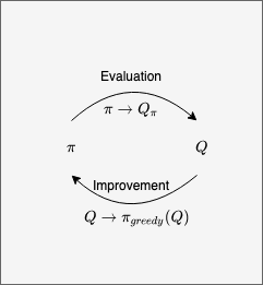
Generalized Policy Interaction (GPI)
Other algorithms below will define their own Policy Evaluation stage, and reuse the Policy Improvement stage. This algorithm, alternating between evaluation and improvement until the policy \(\pi\) stops changing, is called Generalized Policy Interaction (GPI).
In DP, the Policy Improvement used state-value \(V(s)\) as input, and needed to know the model \(p(s' \vert s, a)\) in step 5. Other algorithms, e.g. SARSA, Q-learning, will feed action-values \(Q(s, a)\) to the Policy Improvement stage, and thus are model-free in their Policy Improvement.
Temporal Difference Algorithms
This is a family of algorithms: TD0, TD(n), TD(\(\epsilon\)). For Temporal Dif ference algorithms, we do not assume that the model \(p(s' \vert s, a)\) is known. The Policy Improvement step is same as for DP. The Policy Evaluation step for \(V_\pi(s)\) is different.
We pick a weight factor \(0 \lt \alpha \le 1\) and a number of episodes \(MAX\_EPISODES\). We will iterate over tragectories \(\tau = s_0, a_0, ..., s_T, a_T\), estimating \(V_\pi(s_t)\) at each step with a value \(G_{\tau, \pi}(s_t)\), and replacing \(V_\pi(s_t) \leftarrow V_\pi(s_t) + \alpha (G_{\tau, \pi}(s_t) - V_\pi(s_t))\).
TD Algorithm
For the TD0 algorithm, \(G_{\tau, \pi}(s_t) \leftarrow r(s_t, a_t) + \gamma V_\pi(s_{t+1})\). The algorithm is:
\(~~~~\) 1: Policy Evaluation for \(\pi\):
\(~~~~~~~~\) 2: Initialize all \(V_\pi(s)\) to random values
\(~~~~~~~~\) 3: For each episode \(0, 1, ..., MAX\_EPISODES-1\):
\(~~~~~~~~~~~~\) 4: Pick \(s_0 \in \mathcal{S}\)
\(~~~~~~~~~~~~\) 5: For \(t=0, ..., T-1\)
\(~~~~~~~~~~~~~~\) 6: Set \(a_t \leftarrow\) action given by \(\pi\) for \(s_t\)
\(~~~~~~~~~~~~~~\) 7: Take action \(a_t\), observe \(r(s_t, a_t)\), \(s_{t+1}\)
\(~~~~~~~~~~~~~~\) 8: Set \(G_{\tau, \pi}(s_t) \leftarrow r(s_t, a_t) + \gamma V_\pi(s_{t+1})\)
\(~~~~~~~~~~~~~~\) 9: Set \(V_\pi(s_t) \leftarrow V_\pi(s_t) + \alpha (G_{\tau, \pi}(s_t) - V_\pi(s_t))\)
\(~~~~\) 10: Policy Update of \(\pi\): Same as for DP
In step 9, the value \(V_\pi(s_t)\) is updated with a weighted average between itself and the discounted value of the next step. At the end of steps 1-9, we get an estimate of \(V_\pi(s)\) for the policy \(\pi\), and can update \(\pi\) using the same Policy Improvement algorithm from DP, switching back and forth between Policy Evaluation and Policy Improvement until the policy \(\pi\) stops changing.
The Policy Evaluation stage of TD is model-free. The GPI stage is not, because DT feeds in the state-vaue function \(V(s)\) to the Policy Update step.
TD(n) Algorithm
A variant TD(n) of the TD algorithm changes step 5 to sample the entire trajectory at once, and changes step 8 to use the weighted average with the discounted value of the next \(n\) steps:
\[\begin{align} G_{\tau, \pi}(s_t) \leftarrow r(s_t, a_t) + \gamma V_\pi(s_{t+1}) + ... + \gamma^{n-1} V_\pi(s_{t+n}) \end{align}\]TD(\(\epsilon\)) Algorithm
Another variant TD(\(\epsilon\)) of TD changes the Policy Evaluation stage to apply it to an \(\epsilon\)-greedy modification of \(\pi\), denoted \(\pi_\epsilon\), which picks in state \(s\) the action \(a\) with probability \((1 - \epsilon)\pi(a \vert s)\), and randomly with likelyhood \(\epsilon\). The \(\epsilon\)-greedy action selection policy balances exploration, with likelihood \(\epsilon\), and exploitation with likelihood \(1-\epsilon\).
Q-Learning and SARSA
The Policy Improvement step for these algorithms is also same as for DP. But, rather than learn the value function \(V_\pi(s)\), the Q-Learning and SARSA algorithms learn directly the action-vaue function \(Q_\pi(s, a)\), and pass that as input to the Policy Improvement stage.
These algorithms can be thought to update the action-value table below, based on the policy \(\pi\); then, they update the policy \(\pi\) based on the table, and iterate the process until the policy \(\pi\) stops changing.
| \(a_0\) | \(a_1\) | … | \(a_{n-1}\) | |
|---|---|---|---|---|
| \(s_0\) | \(Q(s_0, a_0)\) | \(Q(s_0, a_1)\) | \(Q(s_0, a_{n-1})\) | |
| \(s_1\) | \(Q(s_1, a_0)\) | \(Q(s_1, a_1)\) | \(Q(s_1, a_{n-1})\) | |
| … | … | … | … | |
| \(s_{m-1}\) | \(Q(s_{m-1}, a_0)\) | \(Q(s_{m-1}, a_1)\) | \(Q(s_{m-1}, a_{n-1})\) |
The policy \(\pi\) can be immediately be updated from the table, because \(Q(s, a)\) is already computed.
In both algorithms, the table is randomly initialized with numbers \(Q(s, a)\).
We pick a weight factor \(0 \lt \alpha \le 1\), a small number \(0\le \epsilon <1\), and a number of episodes \(MAX\_EPISODES\). We will iterate over tragectories \(\tau = s_0, a_0, ..., s_T, a_T\), estimating \(Q_\pi(s_t, a_t)\) at each step with a value \(G_{\tau, \pi}(s_t, a_t)\), replacing \(\begin{align} Q_\pi(s_t, a_t) \leftarrow Q_\pi(s_t, a_t) + \alpha (G_{\tau, \pi}(s_t, a_t) - Q_\pi(s_{t+1}, a_{t+1})) \end{align}\)
For SARSA, \(G_{\tau, \pi}(s_t, a_t) \leftarrow r(s_t, a_t) + \gamma Q_\pi(s_t, a_t)\).
For Q-Learning, \(G_{\tau, \pi}(s_t, a_t) \leftarrow r(s_t, a_t) + \gamma \, \underset{a \in \mathcal{A}}{max} \, Q_\pi(s_{t+1}, a)\).
SARSA
\(~~~~\) 1: Initialize all \(Q_\pi(s, a)\) to random values
\(~~~~\) 2: Policy Evaluation for \(\pi\):
\(~~~~~~\) 3: For each episode \(0, 1, ..., MAX\_EPISODES-1\):
\(~~~~~~~~\) 4: Pick a trajectory \(\tau = s_0, a_0, ..., s_T, a_T\) using \(\pi\) (or \(\pi_\epsilon\))
\(~~~~~~~~\) 5: For each \(0 \le t \lt T\)
\(~~~~~~~~~~\) 6: Set \(G_{\tau, \pi}(s_t, a_t) \leftarrow r(s_t, a_t) + \gamma Q_\pi(s_{t+1}, a_{t+1})\)
\(~~~~~~~~~~\) 7: Set \(Q_\pi(s_t, a_t) \leftarrow Q_\pi(s_t, a_t) + \alpha (G_{\tau, \pi}(s_t, a_t) - Q_\pi(s_t, a_t))\)
\(~~~~\) 8: Policy Update of \(\pi\): Same as for DP
It is called SARSA because the update step 6 depends on \(s_t, a_t, r, s_{t+1}, a_{t+1}\). We could always use \(T = 2\) in SARSA.
This algorithm is model-free but on-policy, because step 4 depends on \(Q_\pi(s_{t+1}, a_{t+1})\), which is policy-specific.
The n-step method TD(n) idea - having the function \(G_{\tau, \pi}(s_t, a_t)\) estimate use n forward steps instead of one - can be extended to SARSA as well.
Q-Learning
This algorithm is same as SARSA but \(G_{\tau, \pi}(s_t, a_t) \leftarrow r(s_t, a_t) + \gamma \, \underset{a \in \mathcal{A}}{max} \, Q_\pi(s_{t+1}, a)\).
Notice that \(G_{\tau, \pi}(s_t, a_t)\) for Q-Learning is not policy-specific. The only step depending on the policy is the choice of trajectory \(\tau\).
However, Q-learning could be used even when the trajectory \(\tau\) was sampled with a different policy (as long as it is not ‘much too different’ from the policy being learned, loosely speaking).
Since Q-learning could be performed on data gathered earlier by another policy, it is an off-policy algorithm.
ML algorithms: SARSA, DQN
The algorithms above still assume a small number of states. When the number of states is large, neural networks come to the rescue to approximate the action-value functions \(Q_\pi(s, a)\).
The setup is the same for the ML version of SARSA and for DQN. We construct a deep neural network with states \(s \in \mathcal{S}\) as input, and action-value functions \(Q(s, a)\) outputs for all actions \(a \in \mathcal{A}\).

Denote \(w\) the weights of the NN, and \(Q_w(s, a)\) the output of the NN. Initialize a learning rate \(\alpha\).
ML SARSA
\(~~~~\) 1: Initialize \(\epsilon > 0\)
\(~~~~\) 2: Randomly initialize the network weights \(w\)
\(~~~~\) 3: For each episode \(0, 1, ..., MAX\_EPISODES-1\):
\(~~~~~~\) 4: Pick N trajectories \(s_i, a_i, s'_i, a'_i\) using the current policy \(\pi_\epsilon\)
\(~~~~~~\) 5: # Calculate NN loss
\(~~~~~~\) 6: \(L(w) \leftarrow \frac{1}{N}\sum_{i=0}^{N-1} \big(Q_w(s_i, a_i) - r(s_i, a_i) - \gamma Q_w(s'_i, a'_i)\big)^2\)
\(~~~~~~\) 7: # Update the network parameters using gradient descent
\(~~~~~~\) 8: \(w \leftarrow w - \alpha \nabla_{w} L(w)\)
\(~~~~~~\) 9: Decay \(\epsilon\)
Like its non-ML counterpart, ML SARSA is on-policy because at step 6 it employ \(Q_w(s'_i, a'_i)\) which depends on the policy implied by the NN weights \(w\).
To improve the performce, ML-SARSA can save in step 8 the adjusted weights \(w\), and only apply an average adjustment after a batch of episodes. This technique is an example of on-policy batched memory replay. Aternatively, the weight adjustments for a batch of episodes can be applied all at once.
Instead of an \(\epsilon\)-greedy policy \(\pi_\epsilon\) in step 4, one can use a Boltzmann policy \(\pi_{boltzmann}\) which, in state \(s\), favors random selection of states \(s'\) sampled by higher action-valie \(Q_\pi(s', a')\). With the Bolzmann policy, actions are sampled according to the distribution
\[\begin{align} p_{bolzmann}(a \vert s) = \frac{e^{Q_\pi(s, a)/\tau}}{\sum_{a'}e^{Q_\pi(s, a)/\tau}} \end{align}\]The temperature factor \(\tau\) in the Bolzmann policy is decayed in step 9 of the algorithm. As \(\tau\) approaches 0, \(p_{bolzmann}(a \vert s)\) converges to 1 for actions \(a\) that maximize \(Q_\pi(s, a)\).
The DQN algorithm
It is similar to SARSA, except that
- In step 4, we pick only a trajectory \(s_i, a_i, s'_i\)
- In step 6, the network loss function is updated according to the Q-learning method \(L(w) \leftarrow \frac{1}{N}\sum_{i=0}^{N-1} \big(Q_w(s_i, a_i) - r(s_i, a_i) - \gamma \underset{a'_i}Q_w(s'_i, a'_i)\big)^2\)
Furthermore, batch memory replay for DQN can emply a much larger buffer of weight updates - between 10,000 and 1,000,000 - because DQN is off policy, and does not have to only use recent memory replays like SARSA.
DQN References:
- Human-level control through deep reinforcement learning, V. Mnih et al, Nature(2015). See p. 3 for DQN performance on Atari games compared with human-level.
- Deep Q Network (DQN), J. Torres (2020): example implementation using Torch